... mit Hilfe der Wellengleichung

Qualität und Rechenzeit

H. Rist
Unsere Gesellschaft bietet seit einiger Zeit die Migration mit der Wellengleichung an (vergl. Artikel von W. Houba im PRAKLA-SEISMOS-Report 1/76). Die Ergebnisse mit diesem Verfahren sind - das wissen wir inzwischen - sehr zufriedenstellend. Dem Verfahren geht allerdings der Ruf voraus, daß es rechenzeitaufwendig und darum teuer ist.
Deshalb sollen hierzu ein paar klärende Erläuterungen gegeben werden.

Es erscheint plausibel, daß die bessere Qualität des Migrationsergebnisses eine längere Rechenzeit erfordert und darum teuer ist. Gute Qualität ist erwünscht, lange Rechenzeit keineswegs. Es geht also darum, einen optimalen Kompromiß zu finden, der bei zufriedenstellender Qualität eine tragbare Rechenzeit erfordert.

Das PRAKLA-SEISMOS-Programm für die Migration mit der Wellengleichung arbeitet im GEOPLAN-System. Die Konzeption des Migrations-Verfahrens gestattet es, mit nur einem einzigen Parameter den Programmablauf zu steuern. Alle anderen Eingabedaten sind die bei anderen Programmabläufen üblichen Angaben, die sich auf das Profil und die Art der Darstellung beziehen. Dieser eine Parameter ist die Tiefenschrittweite Δ z.

Die "natürliche" Tiefenschrittweite wäre eine der Sampling Rate entsprechende Schrittweite Δ z = Δt.vort (vort = Ortsgeschwindigkeit). Man müßte dann ebensoviel " Etagen" (Ebenen, in denen die Geophone gedanklich plaziert sind, siehe Artikel W. Houba im Report 1/76) in die Tiefe rechnen, wie eine Spur Sampies hat, und das ist meist eine beträchtliche Menge; lange Rechenzeiten wären die Folge. Hierbei würde man jedoch mit einer "Genauigkeit" rechnen, die nur in der Theorie existiert, die aber wegen unvermeidbarer Ungenauigkeiten in anderen Parametern - z.B. bei den Geschwindigkeiten - niemals realisiert werden kann. Ein derartiger Rechenzeitaufwand wäre daher sinnlos.

Aus diesem Grunde rechnet man mehrere Etagen gemeinsam in einem einzigen Rechengang auf eine mittlere (zentrale) Tiefe und hat damit die Möglichkeit, die Rechenzeit beträchtlich zu verkürzen. Die Anzahl der gleichzeitig gerechneten Etagen nennt man die in Sampies gemessene Tiefenschrittweite Δz. Man kann sie auch in ms angeben, was den Vorzug der größeren Anschaulichkeit hat. Die Tendenz der Abhängigkeit der Rechenzeit von der Tiefenschrittweite Δz ist in Fig. 1 dargestellt.

In die Rechenzeit geht, abgesehen von einem Zeitanteil für die Ein-und Ausgabe und eventuelle Routineprozesse, die Anzahl der Sampies pro Spur quadratisch ein.

Die Anzahl der Spuren hat auf die benötigte Rechenzeit einen weitaus geringeren Einfluß.

...using wave equation

Quality and Computing Time

Our company is presently offering the migration process using wave-equation (see W. Houba's article in the PRAKLA-SEISMOS Report 1/76). The results obtained with this procedure are - according to our experience highly satisfactory. However, this procedure is reputed to be time-consuming and thus too expensive. We therefore wish to make a couple of explanatory remarks.

It seems plausible that a better quality migration result requires more computing time, thus making the process more expensive. Good quality is wanted, long computing time not at all. The point is thus to find an optimum compromise which is of satisfactory quality and requires only reasonable computing time.

The PRAKLA-SEISMOS migration program using the wave-equation operates in the GEOPLAN-system. The design of the migration procedure permits control of the program run with only one single parameter. All other input data are those which are generally used in other program runs, dealing with the line data and the type of display. This sole parameter is the depth step width Δz.

The "natural" depth step width would be a step width Δz = Δt.vinst (vinst = instantenous velocity), corresponding to the sampling rate. So, as many "levels" (the planes ' on which the geophones are thought to be placed, see article W. Houba, Report 1/76) would have to be calculated downwards as a trace has sampies, and this is generally a considerable quantity; large computing time would be the consequence. However, one would be computing with an "accuracy" which is only existent in theory, but which because of unavoidable inaccuracies in other parameters - e. g. in velocities - can never be realized. Such a computer time consumption would there fore be useless.

Fig. 1 Abhängigkeit der Rechenzeit von der Tiefenschrittweite Δz
Dependence of computing time on the step width Δz

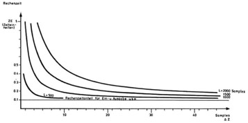
Bei einer im Zeitmaßstab gemessenen Seismogrammlänge von 2000 ms und einer Tiefenschrittweite von 5 Samples (20 ms bei 4 ms Sampling Rate) beträgt der Focussierungsfehler (Abweichung von dem theoretisch genauen Migrationspunkt) höchstens ± 2 Sampies (± 10 ms). Das entspricht einem relativen Fehler von 0,5% in Bezug auf die Gesamtlänge von 2000 ms. Die Rechenzeitverkürzung auf etwa ein Fünftel gegenüber der Rechenzeit bei einer Tiefenschrittweite von 4 ms rechtfertigt den Verzicht auf eine nur vorgetäuschte aber in der Praxis nicht erreichbare Genauigkeit.

For this reason levels are calculated downwards in packages furnishing a "centralized" level with several adjacent levels, thus reducing considerably the computing time needed. The number of simultaneously cal culated levels is called depth step width Δz, measured in samples. For the sake of clarity, however, it is usually given in ms. The dependence of computing time on the depth step width Δz is presented in Fig. 1.

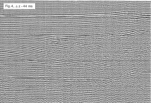
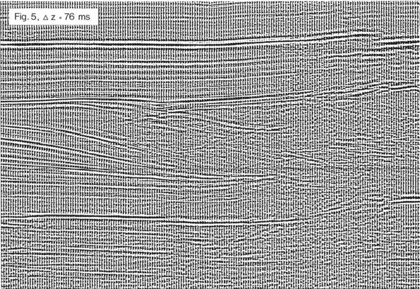
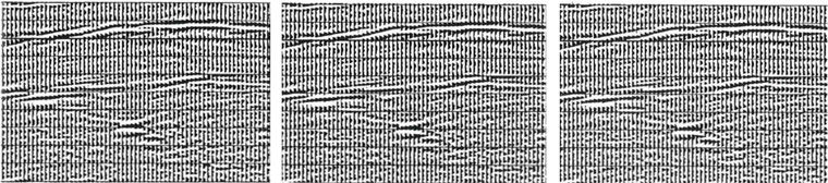
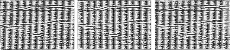
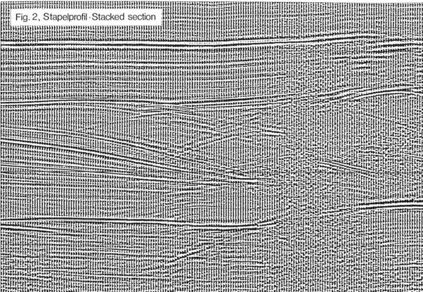
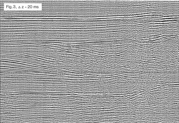
Die Figuren 3 bis 7 zeigen jeweils denselben Profilauschnitt des Stapelprofils in Figur 2 der jedoch mit ver- schiedenen Tiefenschrittweiten migriert wurde. Man erkennt, daß bei den Tiefenschrittweiten 20 ms und 44 ms kaum ein Qualitätsunterschied besteht, während bei der nächsten Tiefenschrittweite von 76 ms in einigen Bereichen eine Qualitätsminderung zu verzeichnen ist. Die Tiefenschrittweiten von 148 ms und 292 ms haben eine merklich schlechtere Qualität.

Apart from a certain time necessary for input/output and possible routine processes, the number of sampies per trace enters quadratically into the computing time. The number of traces has a much lower influence on the computing time required.

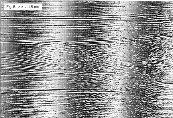
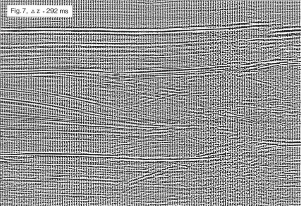
In Figur 7 (Δ = 292 ms) sind zwar die Diffraktionen an den Störungen noch etwas schwächer als im Stapelprofil, die Reflexionsqualität hat sich aber in den schrägen Horizonten sogar verschlechtert.

At a seismogram length of 2000 ms and a depth step width of 5 sampies (20 ms at 4 ms sampling rate) the focusing error (deviation of the theoretically exact migration point) is max. of ± 2 sampies (± 10 ms). This corresponds to a relative error of 0,5% with respect to the total length of 2000 ms. The reduction of computing time to about a fifth, compared to the computing time at a depth step width of 4 ms, thus justifies forgoing a theoretically possible but in practice not attainable accuracy.

Fig.8
Stapelprofil mit
ausgeprägter Kleintektonik.
Die Figuren 9 bis 15
entsprechen dem hier
eingerahmten Profilausschnitt.

Stacked section with
characteristic minor tectonics.
The figures 9 to 15 correspond
to the rectangularly framed part
of this section.

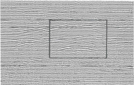
Fig. 8, Slapelprofil . Slacked seclion

Fig. 9, Δz = 12 ms

Figs. 3-7 present the same section of the stacked line in Fig. 2 which, however, was migrated with different depth step widths. One recognizes that there is hardly any difference in quality at the step widths 20 ms and 44 ms, whereas at the next depth step width of 76 ms there is a decrease in quality in some regions. The depth step widths of 148 ms and 292 ms have a noticeably worse quality. As to Fig. 7 (Δz = 292 ms) the diffractions at faults are somewhat weaker than in the stacked line, the reflection quality, however, decreased in dipped horizons.

In einer zweiten Versuchsreihe wurde die Abhängigkeit der Migrationsqualität von den Tiefenschrittweiten in einem Profil mit ausgeprägter Kleintektonik untersucht. Nach der Migration wird an einer Stelle, die im Stapelprofil Figur 8 rechteckig eingerahmt ist, eine mehr oder weniger gut ausgebildete kleine Mulde sichtbar. Die Mulde wurde aus dem Gesamtprofil "herausgeschnitten" und in den Figuren 9 bis 15 - entsprechend den Δ z-Schritten 12 ms, 20 ms, 36 ms, 52 ms, 100 ms, 148 ms und 196 ms abgebildet. Man sieht, daß bei den Δz-Schritten 12 ms, 20 ms, 36 ms und sogar noch 52 ms die Reflexionsqualität, vor allem die der Muldenflanken, gleich ist. Erst ab Δz = 100 ms verwischen sich die Flanken und in den beiden letzten Migrationen mit den Schritten 148 ms und 196 ms ist die Mulde fast verschwunden.

The dependence of migration quality on the depth step widths has been also investigated in a line with characteristic small tectonics in a second test. After migration, a more or less weil defined sma/l trough is visible at a point which is rectangularly framed in the stacked line of Fig. 8. The trough was "cut out" from the total section and imaged in Figs. 9-15, corresponding to the Δz-steps 12 ms, 20 ms, 36 ms, 52 ms, 100 ms, 148 ms and 196 ms. One recognizes that in the Δz-steps 12 ms, 20 ms, 36 ms and even 52 ms the reflection quality, especially that of the through-flanks, is the same. Only from Δz = 100 ms the flanks become blurred, and in the two last migrations with the steps 148 ms and 196 ms the trough nearly disappears.

Die optimale Arbeitsweise liegt in einem Bereich, wo bei zunehmendem Δ.z der Qualitätsverlust gering, der Rechenzeitgewinn jedoch bedeutend ist: es ist der Bereich, in dem die Kurven der Figur 1 flach werden. Dieser günstige Bereich ist verhältnismäßig unkritisch. Er liegt, je nach Nutzfrequenzen und Neigung, ungefähr zwischen Tiefenschrittweiten von 20 und 48 ms. Nach den bisherigen Erfahrungen führt das Programm in diesem Bereich zu einem kaum zu verbessernden Ergebnis. PRAKLA-SEISMOS bietet die Migration mit der Weilengleichung bei Tiefenschrittweiten zwischen 20 und 50 ms zu Preisen an, die etwa denen der kohärenzgewichteten Diffraktionsmigration entsprechen. Bei Tiefenschrittweiten über 50 ms sind die Migrationskosten entsprechend geringer.

The optimum procedure lies in a range where at increasing Δ.z the quality loss is low, yet the gain of computing time is significant: it is the range where the curves of Fig. 1 are flattened out. This favourable range is relatively uncritical. It is located, depending on frequencies and dip, approximately between the depth step widths of 20 and 48 ms. According to our experience the program leads in this range to results that can hardly be improved. PRAKLA-SEISMOS offers the migration process using wave equation at depth step widths between 20 and 50 ms at prices which approximately correspond to those of coherency-weighted diffraction migration. At step widths mor than 50 ms the migration costs are accordingly lower.